NN Learning
We can solve for gradients in a vectorized manner.
A function \(\mathbf{f}: R^n \xrightarrow{} R^m\) exists such that \(\mathbf{f}(\mathbf{x}) = [f_1(x_1, ..., x_n), f_2(x_1, ..., x_n), ..., f_m(x_1, ..., x_n)]\). Its jacobian can be calculated as
In other words, \((\frac{d\mathbf{f}}{d\mathbf{x}})_{ij} = \frac{df_i}{dx_j}\). This jacobian is useful for the application of chain rule to a vector-valued function just by multiplying jacobians.
For example, suppose we have a function \(\mathbf{f}(x) = [f_1(x), f_2(x)]\) taking a scaler to a vector of size 2 and a function \(\mathbf{g}(\mathbf{y}) = [g_1(y_1, y_2), g_2(y_1, y_2)]\) taking a vector of size two to a vector of size two. Now let’s compose them to get \(\mathbf{g}(x) = [g_1(f_1(x), f_2(x)), g_2(f_1(x), f_2(x))]\). Using the regular chain rule, we can compute the derivative of \(\mathbf{g}\) as the Jacobian
This is the same as multiplying the two jacobians.
Useful Linear Algebra Identities
(1) Matrix times column vector wrt the column vector
\(\mathbf{z} = \mathbf{W} \mathbf{x}\), what is \(\frac{d\mathbf{z}}{d\mathbf{x}}\)?
Suppose \(\mathbf{W} \in R^{n \times m}\), then we can think of z as a function of \mathbf{x} taking an \(m\)-dimensional vector to an \(n\)-dimensional vector. So, its Jacobian will be \(n \times m\). Note that
An entry \((\frac{d\mathbf{f}}{d\mathbf{x}})_{ij}\) of the Jacobian will be
because \(\frac{d}{d x_j} x_k = 1\) if \(k = j\) and 0 if otherwise. So, we see that \(\frac{d \mathbf{z}}{d \mathbf{x}} = \mathbf{W}\).
(2) Row vector times matrix wrt the row vector
\(\mathbf{z} = \mathbf{x} \mathbf{W}\), what is \(\frac{d \mathbf{z}}{d \mathbf{x}}\)?
A computation similar to (1) shows that \(\frac{d \mathbf{z}}{d \mathbf{x}} = \mathbf{W}^T\).
(3) A vector with itself
\(\mathbf{z} = \mathbf{x}\), what is \(\frac{d \mathbf{z}}{d \mathbf{x}}\)?
We have \(z_i = x_i\), so
So we see that the Jacobian \(\frac{d\mathbf{z}}{d \mathbf{x}}\) is a diagonal matrix where the entry at \((i, i)\) is 1. This is just the identity matrix: \(\frac{d\mathbf{z}}{d \mathbf{x}} = \mathbf{I}\). When applying the chain rule, this term will disappear because a matrix or vector multiplied by the identity matrix does not change.
(4) An elementwise function applied a vector
\(\mathbf{z} = f(\mathbf{x})\), what is \(\frac{d \mathbf{z}}{d \mathbf{x}}\)?
Since \(f\) is being applied elementwise, we have \(z_i = f(x_i)\). So,
So we see that the jacobian \(\frac{d\mathbf{z}}{d\mathbf{x}}\) is a diagonal matrix where the entry at \((i,i)\) is the derivative of \(f\) applied to \(x_i\). We can write this as \(\frac{d \mathbf{z}}{d \mathbf{x}} = diag( f^\prime (\mathbf{x}))\). Since multiplication by a diagonal matrix is the same as doing elementwise multiplication by the diagonal, we could also write \(\circ f^\prime (\mathbf{x})\) when applying the chain rule.
(5) Matrix times column vector wrt the matrix
\(\mathbf{z} = \mathbf{W} \mathbf{x}\), \(\mathbf{\delta} = \frac{d J}{d z}\) what is \(\frac{dJ}{d\mathbf{W}} = \frac{d J}{d \mathbf{z}} \frac{d \mathbf{z}}{d \mathbf{W}} = \delta \frac{d \mathbf{z}}{d \mathbf{W}}\)?
Suppose we ahve a loss function \(J\) (a scalar) and are computing its gradient wrt a matrix \(\mathbf{W} \in R^{n \times m}\). Then we could think of \(J\) as a function of \(\mathbf{W}\) taking \(n m\) inputs (the entries of \(\mathbf{W}\)) to a single output (\(J\)). This means the Jacobian \(\frac{d J}{d \mathbf{W}}\) would be a \(1 \times nm\) vector. But in practice this is not a very useful way of arranging the gradient. It would be much nicer if hte derivatives were in a \(n \times m\) matrix like this:
Since this matrix has the same shape as \(\mathbf{W}\), we could just subtract it (times the learning rate) from \(\mathbf{W}\) when doing gradient descent. So (in a slight abuse of notation) let’s find this matrix as \(\frac{d J}{d \mathbf{W}}\) instead.
This way of arranging the gradients becomes complicated when computing \(\frac{d \mathbf{z}}{d \mathbf{W}}\). Unlike \(J\), \(\mathbf{z}\) is a vector. So if we are trying to rearrange the gradients like with \(\frac{d J}{d \mathbf{W}}\), \(\frac{d \mathbf{z}}{d \mathbf{W}}\) would be an \(n \times m \times n\) tensor! Luckily, we can avoid the issue by taking the gradient wrt a single weight \(W_{ij}\) instead. \(\frac{d \mathbf{z}}{d W_{ij}}\) is just a vector, which is much easier to deal with. We have
Note that \(\frac{d}{d W_{ij}} W_{kl} = 1\) if \(i=k\) and \(j=l\) and 0 if otherwise. So if \(k \neq i\) everything in the sum is zero and the gradient is zero. Otherwise, the only nonzero element of hte sum is when \(l=j\), so we just get \(x_j\). Thus we find \(\frac{d z_k}{d W_{ij}} = x_j\) if \(k = i\) and 0 if otherwise. Another way of writing this is
Here, the \(x_j\) is located in the \(i\)th element.
Now let’s compute \(\frac{d J}{d W_{ij}}\)
The only nonzero term in the sum is \(\delta_i \frac{d z_i}{d W_{ij}}\). To get \(\frac{d J}{d \mathbf{W}}\) we want a matrix where entry \((i, j)\) is \(\delta_i x_j\). This matrix is equal to the outer product \(\frac{d J}{d \mathbf{W}} = \delta^T x^T\).
(6) Row vector time matrix wrt the matrix
\(\mathbf{z} = \mathbf{x} \mathbf{W}\), \(\mathbf{\delta} = \frac{d J}{d z}\) what is \(\mathbf{d J}{d \mathbf{W}} = \delta \frac{d \mathbf{z}}{d \mathbf{W}}\)?
A similar computation to the one above shows \(\frac{d J}{d \mathbf{W}} = \mathbf{x}^T \delta\).
(7) Cross-entropy loss wrt logits
\(\mathbf{\hat{y}} = softmax(\mathbf{\theta}), J = CE(\mathbf{y}, \mathbf{\hat{y}})\), what is \(\frac{d J}{d \mathbf{\theta}}\)?
The gradient is \(\frac{d J}{d \mathbf{\theta}} = \mathbf{\hat{y}} - \mathbf{y}\), or \((\mathbf{\hat{y}} - \mathbf{y})^T\) if \(\mathbf{y}\) is a column vector.
These identities will be enough to let you quickly compute the gradients for many neural networks.
Gradient layout
Jacobean formulation is great for applying the chain rule: simply multiply the Jacobians. However, when doing SGD it’s more convenient to follow the convention “the shape of the gradient equals the shape of the parameter” (as done when computing \(\frac{d J}{d \mathbf{W}}\)) That way subtracting the gradient times the learning rate from the parameters is easy.
Example on 1-layer NN
We compute the gradients of a full neural network with one-layer and cross-entropy (CE) loss.
The forward pass is as follows:
It helps to break up the model into the simplest parts possible, so note that we defined \(\mathbf{z}\) and \(\mathbf{\theta}\) to split up the activation functions from the linear transformations in the network’s layers. The dimensions of the model’s parameters are
where \(D_x\) is the size of our input, \(D_h\) is the size of our hidden layer, and \(N_c\) is the number of classes.
In this example, we will compute all of the network’s gradients: \(\frac{d J}{d \mathbf{U}}\), \(\frac{d J}{d \mathbf{b_2}}\), \(\frac{d J}{d \mathbf{W}}\), \(\frac{d J}{d \mathbf{b_1}}\), \(\frac{d J}{d \mathbf{x}}\)
To start with, recall that ReLU(\(x\)) = max(\(x, 0\)). This means
where sgn is the signum function. Note that we are able to write the derivative of the activation in terms of the activation itself.
Now let’s write out the chain rule for \(\frac{d J}{d \mathbf{U}}\) and \(\frac{d J}{d \mathbf{b_2}}\):
Notice that \(\frac{d J}{d \mathbf{\hat{y}}} \frac{d \mathbf{\hat{y}}}{d \mathbf{\theta}} = \frac{d J}{d \mathbf{\theta}}\) is present in both gradients. This makes the math a bit cumbersome. Even worse, if we’re implementing the model without automatic differentiation, computing \(\frac{d J}{d \mathbf{\theta}}\) twice will be inefficient. So it will help us to define some variables to represent the intermediate derivatives:
These are the error signals passed down to \(\mathbf{\theta}\) and \(\mathbf{z}\) when doing backpropagation. We can compute them as follows:
Per cross-entropy loss wrt logits,
Using the chain rule,
Substituting in \(\mathbf{\delta_1}\),
Using matrix times column vector wrt column vector,
Using elementwise function applied to a vector,
These final objects have the following sizes: \(\frac{d J}{d \mathbf{z}}\) is (\(1 \times D_h\)), \(\mathbf{\delta_1}\) is (\(1 \times N_c\)), \(\mathbf{U}\) is (\(N_c \times D_h\)), and \(sgn(\mathbf{h})\) is (\(D_h\), ).
The error terms can be utilized to compute the gradients.
Using the property that the matrix times column vector wrt matrix,
Using identity matrix and transposing
Using the property that the matrix times column vector wrt matrix,
Using identity matrix and transposing
Using matrix times column vector wrt column vector and transposing
[ ]:
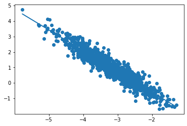
The below example shows the use of backpropagation on a linear regression problem. As a note, this method can be solved (easier, perhaps) with least squares linear algebra.
[36]:
from numpy import *
from sklearn.datasets import make_blobs
import matplotlib.pyplot as plt

# y = mx + b
# m is slope, b is y-intercept
def compute_error_for_line_given_points(b, m, points):
    totalError = 0
    for i in range(0, len(points)):
        x = points[i, 0]
        y = points[i, 1]
        totalError += (y - (m * x + b)) ** 2
    return totalError / float(len(points))

def step_gradient(b_current, m_current, points, learningRate):
    b_gradient = 0
    m_gradient = 0
    N = float(len(points))
    for i in range(0, len(points)):
        x = points[i, 0]
        y = points[i, 1]

        # Calculate gradient with partial derivatives
        m_gradient += -x * (y - (m_current * x + b_current))
        b_gradient += -(y - (m_current * x + b_current))

    new_b = b_current - (learningRate * b_gradient)
    new_m = m_current - (learningRate * m_gradient)
    return [new_b, new_m]

def gradient_descent_runner(points, starting_b, starting_m, learning_rate, num_iterations):
    b = starting_b
    m = starting_m
    for i in range(num_iterations):
        b, m = step_gradient(b, m, array(points), learning_rate)
    return [b, m]

def gen_data():

    n_samples = 1000
    random_state = 170
    X, y = make_blobs(n_samples=n_samples, random_state=random_state, centers=1)

    # Anisotropicly distributed data to stretch the blobs
    transformation = [[0.60834549, -0.63667341], [-0.40887718, 0.85253229]]
    X_aniso = dot(X, transformation)
    return X_aniso

def run():
    points = gen_data()

    learning_rate = 0.0001
    initial_b = 0 # initial y-intercept guess
    initial_m = 0 # initial slope guess
    num_iterations = 1000
    print("Starting gradient descent at b = {0}, m = {1}, error = {2}".format(initial_b, initial_m, compute_error_for_line_given_points(initial_b, initial_m, points)))
    print("Running...")
    [b, m] = gradient_descent_runner(points, initial_b, initial_m, learning_rate, num_iterations)
    print("After {0} iterations b = {1}, m = {2}, error = {3}".format(num_iterations, b, m, compute_error_for_line_given_points(b, m, points)))

    plt.scatter(points[:,0], points[:,1])
    plt.plot(points[:,0], m*points[:,0] + b)
    plt.show()

run()
Starting gradient descent at b = 0, m = 0, error = 2.059703523518794
Running...
After 1000 iterations b = -3.2643663545390273, m = -1.3386872077957057, error = 0.11444715957515363
Rules of thumb for neural networks
Batch normalization standardizes the inputs (or activations of a prior layer or inputs directly), offering some regularization effect and reducing generalization error, perhaps no longer requiring the use of dropout for regularization. It can halve the epochs or better. Do not use dropout and batch normalization at the same time.
The number of hidden layers in a neural network \(N_h = \frac{N_s}{\alpha \times (N_i + N_o)}\) where \(\alpha\) is an arbitrary scaling factor (usually 2 through 10) which symbolizes the number of nonzero weights for each neuron (which is smaller when including dropout layers), \(N_i\) is the number of input neurons, \(N_o\) is the number of output neurons, and \(N_s\) number of samples in a training data set.
[2]:
# -*- coding: utf-8 -*-
import torch
import math


class LegendrePolynomial3(torch.autograd.Function):
    """
    We can implement our own custom autograd Functions by subclassing
    torch.autograd.Function and implementing the forward and backward passes
    which operate on Tensors.
    """

    @staticmethod
    def forward(ctx, input):
        """
        In the forward pass we receive a Tensor containing the input and return
        a Tensor containing the output. ctx is a context object that can be used
        to stash information for backward computation. You can cache arbitrary
        objects for use in the backward pass using the ctx.save_for_backward method.
        """
        ctx.save_for_backward(input)
        return 0.5 * (5 * input ** 3 - 3 * input)

    @staticmethod
    def backward(ctx, grad_output):
        """
        In the backward pass we receive a Tensor containing the gradient of the loss
        with respect to the output, and we need to compute the gradient of the loss
        with respect to the input.
        """
        input, = ctx.saved_tensors
        return grad_output * 1.5 * (5 * input ** 2 - 1)


dtype = torch.float
device = torch.device("cpu")
# device = torch.device("cuda:0")  # Uncomment this to run on GPU

# Create Tensors to hold input and outputs.
# By default, requires_grad=False, which indicates that we do not need to
# compute gradients with respect to these Tensors during the backward pass.
x = torch.linspace(-math.pi, math.pi, 2000, device=device, dtype=dtype)
y = torch.sin(x)

# Create random Tensors for weights. For this example, we need
# 4 weights: y = a + b * P3(c + d * x), these weights need to be initialized
# not too far from the correct result to ensure convergence.
# Setting requires_grad=True indicates that we want to compute gradients with
# respect to these Tensors during the backward pass.
a = torch.full((), 0.0, device=device, dtype=dtype, requires_grad=True)
b = torch.full((), -1.0, device=device, dtype=dtype, requires_grad=True)
c = torch.full((), 0.0, device=device, dtype=dtype, requires_grad=True)
d = torch.full((), 0.3, device=device, dtype=dtype, requires_grad=True)

learning_rate = 5e-6
for t in range(2000):
    # To apply our Function, we use Function.apply method. We alias this as 'P3'.
    P3 = LegendrePolynomial3.apply

    # Forward pass: compute predicted y using operations; we compute
    # P3 using our custom autograd operation.
    y_pred = a + b * P3(c + d * x)

    # Compute and print loss
    loss = (y_pred - y).pow(2).sum()
    if t % 100 == 99:
        print(t, loss.item())

    # Use autograd to compute the backward pass.
    loss.backward()

    # Update weights using gradient descent
    with torch.no_grad():
        a -= learning_rate * a.grad
        b -= learning_rate * b.grad
        c -= learning_rate * c.grad
        d -= learning_rate * d.grad

        # Manually zero the gradients after updating weights
        a.grad = None
        b.grad = None
        c.grad = None
        d.grad = None

print(f'Result: y = {a.item()} + {b.item()} * P3({c.item()} + {d.item()} x)')
99 209.95831298828125
199 144.6602020263672
299 100.70250701904297
399 71.03519439697266
499 50.97850799560547
599 37.403133392333984
699 28.206867218017578
799 21.97317886352539
899 17.745729446411133
999 14.877889633178711
1099 12.93176555633545
1199 11.610918045043945
1299 10.714245796203613
1399 10.105476379394531
1499 9.69210433959961
1599 9.411376953125
1699 9.220744132995605
1799 9.091286659240723
1899 9.003360748291016
1999 8.943641662597656
Result: y = 4.691534383205465e-10 + -2.208526849746704 * P3(2.9543581470115043e-10 + 0.2554861009120941 x)